Basic pipeline for exploratory analysis

Load modules

from robustica import RobustICA, corrmats

import pandas as pd
import numpy as np
from sklearn.utils import parallel_backend

import matplotlib.pyplot as plt
import seaborn as sns

Load data from Sastry (2019)

url = "https://static-content.springer.com/esm/art%3A10.1038%2Fs41467-019-13483-w/MediaObjects/41467_2019_13483_MOESM4_ESM.xlsx"
data = pd.ExcelFile(url)
data.sheet_names

['README',
 'Metadata',
 'Expression Data',
 'S matrix',
 'A matrix',
 'Media Recipes',
 'Gene Information']

data.parse("README")

	Sheet Name	Description
0	Experimental Conditions	Experimental conditions for each sample in PRE...
1	Expression Data	Expression levels of genes (log2 Transcripts p...
2	S matrix	I-modulon gene coefficients. Each column is an...
3	A matrix	Condition-specific i-modulon activities. Each ...
4	Media Description	Recipes for base media and trace element mixtures
5	Gene Information	Mapping of b-numbers to gene names/annotations...
6	NaN	NaN
7	Metadata Columns	Description
8	Sample ID	Unique sample identifier for experiment (e.g. ...
9	Study	Short 1-2 word description of study where samp...
10	Project ID	Identifier for study
11	Condition ID	Identifier for unique experimental conditions
12	Replicate #	Suffix for sample ID to distinguish between re...
13	Strain Description	Describes gene knock-out, mutation knock-in, o...
14	Strain	MG1655 or BW25113
15	Base Media	Media recipe as described in Media Description...
16	Carbon Source (g/L)	Carbon source in g/L
17	Nitrogen Source (g/L)	Nitrogen source in g/L
18	Electron Acceptor	Aerobic (O2), anaerobic (None), or nitrate (KN...
19	Trace Element Mixture	Trace element recipe as described in Media Des...
20	Supplement	Additional media supplements in each experimen...
21	Temperature (C)	Temperature of growth condition in Celsius
22	pH	Neutral (7) or acidic (5.5)
23	Antibiotic	Treatment with low concentration Kanamycin for...
24	Culture Type	Batch or Chemostat (always exponential growth ...
25	Growth Rate (1/hr)	Measured growth rate of strain in media
26	Evolved Sample	Whether the strain was from an adaptive labora...
27	Isolate Type	Clonal or Population (only applicable to ALE s...
28	Sequencing Machine	Type of machine used for sequencing
29	Additional Details	Additional information about experiment
30	Biological Replicates	Number of biological replicates within study
31	Alignment	Percent of reads aligned by bowtie to referenc...
32	DOI	Accession number for study
33	GEO	GEO Accession ID

Preprocess data

Following the article’s methods, we compute the log2FCs with respect to controls

# get gene expression
X = data.parse("Expression Data").set_index("log-TPM")

# get controls
controls = [c for c in X.columns if "control" in c]
print(controls)

# compute log2FCs with respect to controls
X = X - X[controls].mean(1).values.reshape(-1, 1)

X

['control__wt_glc__1', 'control__wt_glc__2']

	control__wt_glc__1	control__wt_glc__2	fur__wt_dpd__1	fur__wt_dpd__2	fur__wt_fe__1	fur__wt_fe__2	fur__delfur_dpd__1	fur__delfur_dpd__2	fur__delfur_fe2__1	fur__delfur_fe2__2	...	efeU__menFentC_ale29__1	efeU__menFentC_ale29__2	efeU__menFentC_ale30__1	efeU__menFentC_ale30__2	efeU__menFentCubiC_ale36__1	efeU__menFentCubiC_ale36__2	efeU__menFentCubiC_ale37__1	efeU__menFentCubiC_ale37__2	efeU__menFentCubiC_ale38__1	efeU__menFentCubiC_ale38__2
log-TPM
b0002	-0.061772	0.061772	0.636527	0.819793	-0.003615	-0.289353	-1.092023	-0.777289	0.161343	0.145641	...	-0.797097	-0.791859	0.080114	0.102154	0.608180	0.657673	0.813105	0.854813	0.427986	0.484338
b0003	-0.053742	0.053742	0.954439	1.334385	0.307588	0.128414	-0.872563	-0.277893	0.428542	0.391761	...	-0.309105	-0.352535	-0.155074	-0.077145	0.447030	0.439881	0.554528	0.569030	0.154905	0.294799
b0004	-0.065095	0.065095	-0.202697	0.119195	-0.264995	-0.546017	-1.918349	-1.577736	-0.474815	-0.495312	...	-0.184898	-0.225615	0.019575	0.063986	0.483343	0.452754	0.524828	0.581878	0.293239	0.341040
b0005	0.028802	-0.028802	-0.865171	-0.951179	0.428769	0.123564	-1.660351	-1.531147	0.240353	-0.151132	...	-0.308221	-0.581714	0.018820	0.004040	-1.228763	-1.451750	-0.839203	-0.529349	-0.413336	-0.478682
b0006	0.009087	-0.009087	-0.131039	-0.124079	-0.144870	-0.090152	-0.219917	-0.046648	-0.044537	-0.089204	...	1.464603	1.415706	1.230831	1.165153	0.447447	0.458852	0.421417	0.408077	1.151066	1.198529
...	...	...	...	...	...	...	...	...	...	...	...	...	...	...	...	...	...	...	...	...	...
b4688	-0.261325	0.261325	-1.425581	-2.734490	0.181893	0.514395	-1.943947	-1.992701	0.066037	-0.695325	...	-0.885297	-0.462485	-2.734490	-1.451148	-1.379069	-1.567420	-0.999610	-1.726577	-2.734490	-1.189069
b4693	-0.278909	0.278909	1.361362	1.020310	0.608108	0.988541	2.558416	2.142724	3.120867	3.104887	...	-0.374963	0.856574	-1.147824	-0.814089	2.054471	1.853620	1.957717	1.943582	2.233115	2.023755
b4696_1	0.050526	-0.050526	1.166436	1.043373	-0.531441	-0.581626	0.914055	0.731165	-0.127269	-0.164046	...	0.261604	0.278426	0.201089	-0.017780	0.138178	0.122287	0.504402	0.425213	0.629383	0.805945
b4696_2	-0.031653	0.031653	0.785573	0.881353	-0.477271	-0.916095	0.837603	0.801393	-0.071710	-0.000540	...	-0.499371	0.398783	0.096609	-0.103446	-0.519098	0.615363	0.343959	0.580288	0.366905	0.702608
b4705	0.724324	-0.724324	-4.350151	-4.317498	-0.747489	-1.257045	-3.308337	-4.421970	-2.679693	-1.872713	...	-1.968530	-1.365300	-5.468290	-2.997169	-3.673367	-3.161608	-3.959910	-4.088644	-5.468290	-5.468290

3923 rows × 278 columns

Run robustica

Using our version of the Icasso algorithm

By default, robustica performs robust ICA by 1. running FastICA multiple times (robust_runs=100) 2. inferring and correcting the signs of components across runs (robust_infer_signs=True) 3. compressing the feature space (rows) (robust_dimreduce=True) 4. using sign-corrected and compressed components to obtain clusters of independent components (robust_method="AgglomerativeClustering" and robust_kws={"linkage": "average"}) 5. uses the clustering labels to compute robust independent components

%%time

rica = RobustICA(n_components=100, robust_runs=8)

with parallel_backend("loky", n_jobs=4):
    S, A = rica.fit_transform(X.values)

print(S.shape, A.shape)

  0%|          | 0/8 [00:00<?, ?it/s]

Running FastICA multiple times...

100%|██████████| 8/8 [00:03<00:00,  2.24it/s]

Inferring sign of components...
Reducing dimensions...
Clustering...
Computing centroids...
(3923, 100) (278, 100)
CPU times: user 3.71 s, sys: 312 ms, total: 4.02 s
Wall time: 7.6 s

Using the classical Icasso algorithm

%%time

rica = RobustICA(
    n_components=100,
    robust_runs=8,
    robust_infer_signs=False,
    robust_dimreduce=False,
    robust_kws={"affinity": "precomputed", "linkage": "average"},
)

with parallel_backend("loky", n_jobs=4):
    S_classic, A_classic = rica.fit_transform(X.values)

print(S_classic.shape, A_classic.shape)

  0%|          | 0/8 [00:00<?, ?it/s]

Running FastICA multiple times...

100%|██████████| 8/8 [00:02<00:00,  3.09it/s]

Precomputing distance matrix...
Clustering...
Computing centroids...
(3923, 100) (278, 100)
CPU times: user 2.38 s, sys: 132 ms, total: 2.51 s
Wall time: 7.51 s

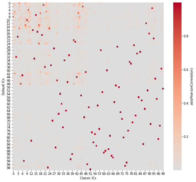
Correspondence between the two approaches

plt.figure(figsize=(11, 10))
sns.heatmap(
    np.abs(corrmats(S.T, S_classic.T)),
    cmap="coolwarm",
    center=0,
    cbar_kws={"label": r"$abs(Pearson Correlation)$"},
)
plt.xlabel("Classic ICs")
plt.ylabel("Default ICs")

plt.show()